
Profiling
Detailed runtime measurements
The tools from the previous section can help us decide the question whether we need to optimize in the first place (is the total run time fast enough?) and it can guide when we want to replace code by a better-performing alternative (such as a more specialized numpy function instead of a general built-in function). They do not tell us what to optimize, though.
As a first example, let’s us have a look at the classical Fibonaci sequence , where each number is the sum of the two preceding numbers. This can be directly written down in a recursive function (note that for simplicity we leave away all error checking, e.g. for negative numbers):
def fibonacci(n):
  if n < 2:
    return n  # fibonacci(0) == 0, fibonacci(1) == 1
  else:
    return fibonacci(n - 2) + fibonacci(n - 1)
This seems to work fine, but the runtime increases with n in a dramatic fashion:
%time factorial(10)CPU times: user 0 ns, sys: 0 ns, total: 0 ns
Wall time: 52.7 µs
89%time factorial(20)CPU times: user 12 ms, sys: 0 ns, total: 12 ms
Wall time: 9.63 ms
10946%time factorial(30)CPU times: user 696 ms, sys: 0 ns, total: 696 ms
Wall time: 695 ms
1346269%time factorial(35)CPU times: user 7.49 s, sys: 24 ms, total: 7.52 s
Wall time: 7.52 s
14930352To get an idea what is going on, we can use %prun, which runs a command with Python’s built-in profiler:
% prun factorial(35)29860706 function calls (4 primitive calls) in 10.621 seconds
Ordered by: internal time
ncalls tottime percall cumtime percall filename:lineno(function)
29860703/1 10.621 0.000 10.621 10.621 <ipython-input-6-b471b8bf6ddb>:1(factorial)
1 0.000 0.000 10.621 10.621 {built-in method builtins.exec}
1 0.000 0.000 10.621 10.621 <string>:1(<module>)
1 0.000 0.000 0.000 0.000 {method 'disable' of '_lsprof.Profiler' objects}The output gives us three pieces of information for every function called during the execution of the command: the number of times the function was called (ncalls), the total time spend in that function itself (tottime) and the time spend in that function, including all time spend in functions called by that function (cumtime). It is not surprising that all of the time is spend in the factorial function (after all, that’s the only function we have) but the function got called 29860703 times! There is no way we are going to get a decent performance from this function without changing the approach fundamentally.
A better Fibonacci sequence
Do you know of a better way to write the Fibonacci function? Can you imagine specific ways of using that function where you would prefer yet another approach?
Optimizing a calculation by using a fundamentally different approach is called “algorithmic optimization” and it is the potentially most powerful way to increase the performance of a program. Whenever the runtime of a program appears to be slow, the first check should be whether there is a function that takes a lot of time and is called more often than expected (e.g. we calculate a measure on 1000 values and expect a function to be called about a 1000 times as well but it is called 1000*1000 times instead).
The output of a profiler run can easily become overwhelming in bigger projects. It can therefore be useful to use a graphical tool that represents this information in a more accessible and interactive way. One such tool is snakeviz that can also be used directly from ipython or a jupyter notebook.
Let’s have a another look at the equalize function we used earlier:
def equalize(image, n_bins=256):
    bins = numpy.linspace(0, 1, n_bins, endpoint=True)
    hist, bins = numpy.histogram(image.flatten(), bins=bins, density=True)
    cdf = hist.cumsum() / n_bins
    # Invert the CDF by using numpy's interp function
    equalized = numpy.interp(image.flatten(), bins[:-1], cdf)

    # All this was performed on flattened versions of the image, reshape the
    # equalized image back to the original shape
    return equalized.reshape(image.shape)
We’ll again load our example image:
image = plt.imread('Unequalized_Hawkes_Bay_NZ.png')[:, :, 0]With snakeviz installed, we can load the snakeviz magic:
%load_ext snakevizWe can then use %snakeviz in the same way we previously used %prun and it will show us a graphical representation of where the time was spent:
%snakeviz equalize(image)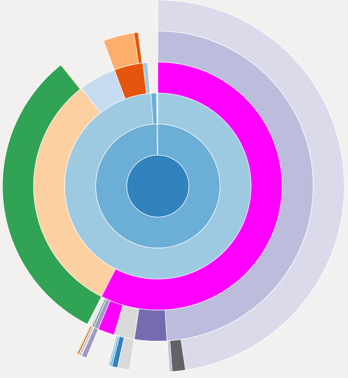
Part of the snakeviz output: A “sunburst” plot showing the runtime spend in various parts of the function call. The center corresponds to the function we are profiling, each layer shows the relative amount of time spend in functions called by functions in the previous layer.
This representation is useful for a global overview of the runtime of the various functions in a project. It might uncover functions that do not seem to be worth optimizing because of their short runtime but are in fact called from various places so that their total runtime is significant.
%prun and %snakeviz give information about which functions take up the most time, but they are less useful to see optimization potential in single functions. Another type of profiling is line-based profiling which measures the runtime of every line in one or more functions. This functionality is provided by the line_profiler package which also provides a magic extension for ipython and the jupyter notebook:
%load_ext line_profilerThe magic command is %lprun and can be used in a similar way to %prun and %snakeviz, but in contrast to those other profiling functions it needs the specification of the functions of interest in addition:
%lprun -f equalize equalize(image)Timer unit: 1e-06 s
Total time: 0.013282 s
File: <ipython-input-96-437a650e3f63>
Function: equalize at line 1
Line # Hits Time Per Hit % Time Line Contents
==============================================================
1 def equalize(image, n_bins=256):
2 1 79 79.0 0.6 bins = numpy.linspace(0, 1, n_bins, endpoint=True)
3 1 8160 8160.0 61.4 hist, bins = numpy.histogram(image.flatten(), bins=bins, density=True)
4 1 18 18.0 0.1 cdf = hist.cumsum() / n_bins
5 # Invert the CDF by using numpy's interp function
6 1 5006 5006.0 37.7 equalized = numpy.interp(image.flatten(), bins[:-1], cdf)
7
8 # All this was performed on flattened versions of the image, reshape the
9 # equalized image back to the original shape
10 1 19 19.0 0.1 return equalized.reshape(image.shape)Note that you can specify several -f function_name arguments to get the information for more than one function with a single %lprun call. For each line, the output specifies how often the line was executed (“Hits”), how long the execution of that line took in total (“Time”) and for each time it was executed (“Per Hit”), and finally how much of the total time of the function was spent in the respective line.